Partial Derivatives, Reverse-Mode Autodiff

A partial derivative measures how much a function changes when you nudge one input, holding every other input fixed. For f(x, y) = x²y + y + 2, the partial derivative with respect to x asks: if y stays put, how fast does f move as x moves?

Manual differentiation

Mathematically, we know that ∂f/∂x = 2xy and ∂f/∂y = x² + 1, using a handful of rules:

• the derivative of a constant is 0
• the derivative of ax is a
• the derivative of x^a is a·x^(a-1)
• the derivative of a sum is the sum of the derivatives: (u + v)' = u' + v'
• the derivative of a product follows the product rule: (u·v)' = u'v + uv'

But how can a program know that?

Reverse-mode Autodiff

The answer is Reverse-mode autodiff — the same technique PyTorch and TensorFlow use.

It break the computation into small steps, run them forward once to get the value, then walk the same steps backward once, applying the chain rule at each step, to get every partial derivative in a single sweep.

Let’s break f(x, y) = x²y + y + 2 into six nodes:

n1 = x
n2 = y
n3 = n1²
n4 = n3 · n2
n5 = n4 + n2
n6 = n5 + 2   (this is f)

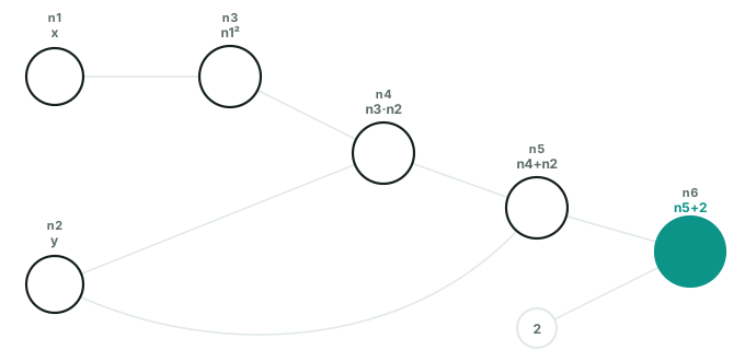
Forward pass: compute the value

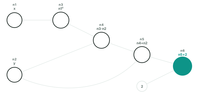
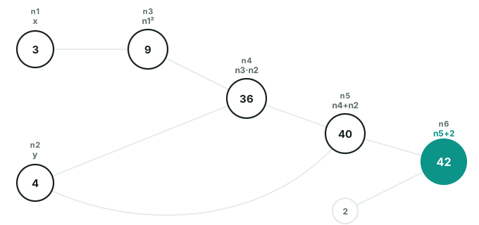
Plug in x = 3, y = 4 and walk the graph left to right, one node at a time. Each node only needs the values of the nodes feeding into it.

n3 = 3² = 9, n4 = 9 · 4 = 36, n5 = 36 + 4 = 40, n6 = 40 + 2 = 42. By the time the graph reaches n6, you have f(3, 4) = 42 — and every intermediate value along the way, kept around for the next pass.

Backward pass: compute the gradient

Now walk the same graph backward, once. At the output, the derivative of f with respect to itself is 1. At every earlier node, multiply the gradient flowing in from the node(s) it feeds by that node’s own local derivative — the chain rule, applied one edge at a time.

Spelled out, one step at a time:

# derivative of f with respect to itself
∂f/∂n6 = 1

# n6 = n5 + 2, so the local derivative ∂n6/∂n5 is 1
# (ax rule for n5, a=1; constant rule for +2, gives 0; sum: 1+0=1)
∂f/∂n5 = ∂f/∂n6 · ∂n6/∂n5
       = 1 · 1
       = 1

# n5 = n4 + n2, so the local derivative ∂n5/∂n4 is 1
# (ax rule for n4, a=1; n2 doesn't depend on n4, gives 0; sum: 1+0=1)
∂f/∂n4 = ∂f/∂n5 · ∂n5/∂n4
       = 1 · 1
       = 1

# n4 = n3 · n2, so the local derivative ∂n4/∂n3 is n2 (product rule)
∂f/∂n3 = ∂f/∂n4 · ∂n4/∂n3
       = 1 · n2
       = 1 · 4
       = 4

# n2 (that's y) feeds both n5 and n4, so sum both paths
# ∂n5/∂n2 = 1 (ax rule), ∂n4/∂n2 = n3 (product rule, symmetric to n3's case)
∂f/∂y  = ∂f/∂n5 · ∂n5/∂n2 + ∂f/∂n4 · ∂n4/∂n2
       = 1 · 1 + 1 · n3
       = 1 · 1 + 1 · 9
       = 1 + 9
       = 10

# n3 = n1², so the local derivative ∂n3/∂n1 is 2·n1 (x^a rule, a=2)
∂f/∂x  = ∂f/∂n3 · ∂n3/∂n1
       = 4 · 2·n1
       = 4 · 2·3
       = 4 · 6
       = 24

Follow the same arithmetic back to n1: ∂f/∂x = 2xy = 24, and ∂f/∂y = x² + 1 = 10 — both computed in a single backward pass.

Why bother with the graph

This is exactly what frameworks like PyTorch and TensorFlow do under the hood, at a much larger scale. One forward pass records the graph; one backward pass computes every partial derivative — no matter how many inputs the function has — for roughly the cost of one extra forward pass. That’s reverse-mode automatic differentiation, and it’s the mechanism that makes training a network with a billion parameters just as mechanical as this six-node example.

Minimal example

Stole from Karpathy’s microgpt example because I feel this Python implementation is neat and serves as a good education purpose.

class Value:
    __slots__ = ('data', 'grad', '_children', '_local_grads')

    def __init__(self, data, children=(), local_grads=()):
        self.data = data                # scalar value of this node calculated during forward pass
        self.grad = 0                   # derivative of the loss w.r.t. this node, calculated in backward pass
        self._children = children       # children of this node in the computation graph
        self._local_grads = local_grads # local derivative of this node w.r.t. its children

    def __add__(self, other):
        other = other if isinstance(other, Value) else Value(other)
        return Value(self.data + other.data, (self, other), (1, 1))

    def __mul__(self, other):
        other = other if isinstance(other, Value) else Value(other)
        return Value(self.data * other.data, (self, other), (other.data, self.data))

    def __pow__(self, other):
        return Value(self.data**other, (self,), (other * self.data**(other-1),))

    def log(self): return Value(math.log(self.data), (self,), (1/self.data,))
    def exp(self): return Value(math.exp(self.data), (self,), (math.exp(self.data),))
    def relu(self): return Value(max(0, self.data), (self,), (float(self.data > 0),))

    def __neg__(self): return self * -1
    def __radd__(self, other): return self + other
    def __sub__(self, other): return self + (-other)
    def __rsub__(self, other): return other + (-self)
    def __rmul__(self, other): return self * other
    def __truediv__(self, other): return self * other**-1
    def __rtruediv__(self, other): return other * self**-1

    def backward(self):
        topo = []
        visited = set()
        def build_topo(v):
            if v not in visited:
                visited.add(v)
                for child in v._children:
                    build_topo(child)
                topo.append(v)
        build_topo(self)
        self.grad = 1
        for v in reversed(topo):
            for child, local_grad in zip(v._children, v._local_grads):
                child.grad += local_grad * v.grad


a = Value(2.0)
b = Value(3.0)
c = a * b       # c = 6.0
L = c + a       # L = 8.0
L.backward()
print(a.grad)   # 4.0 (dL/da = b + 1 = 3 + 1, via both paths)
print(b.grad)   # 2.0 (dL/db = a = 2)

This is exactly what PyTorch’s .backward() gives you:

import torch
a = torch.tensor(2.0, requires_grad=True)
b = torch.tensor(3.0, requires_grad=True)
c = a * b
L = c + a
L.backward()
print(a.grad)   # tensor(4.)
print(b.grad)   # tensor(2.)